Tom Nixon about

Taking a Picture of Sound

30 Dec 2018

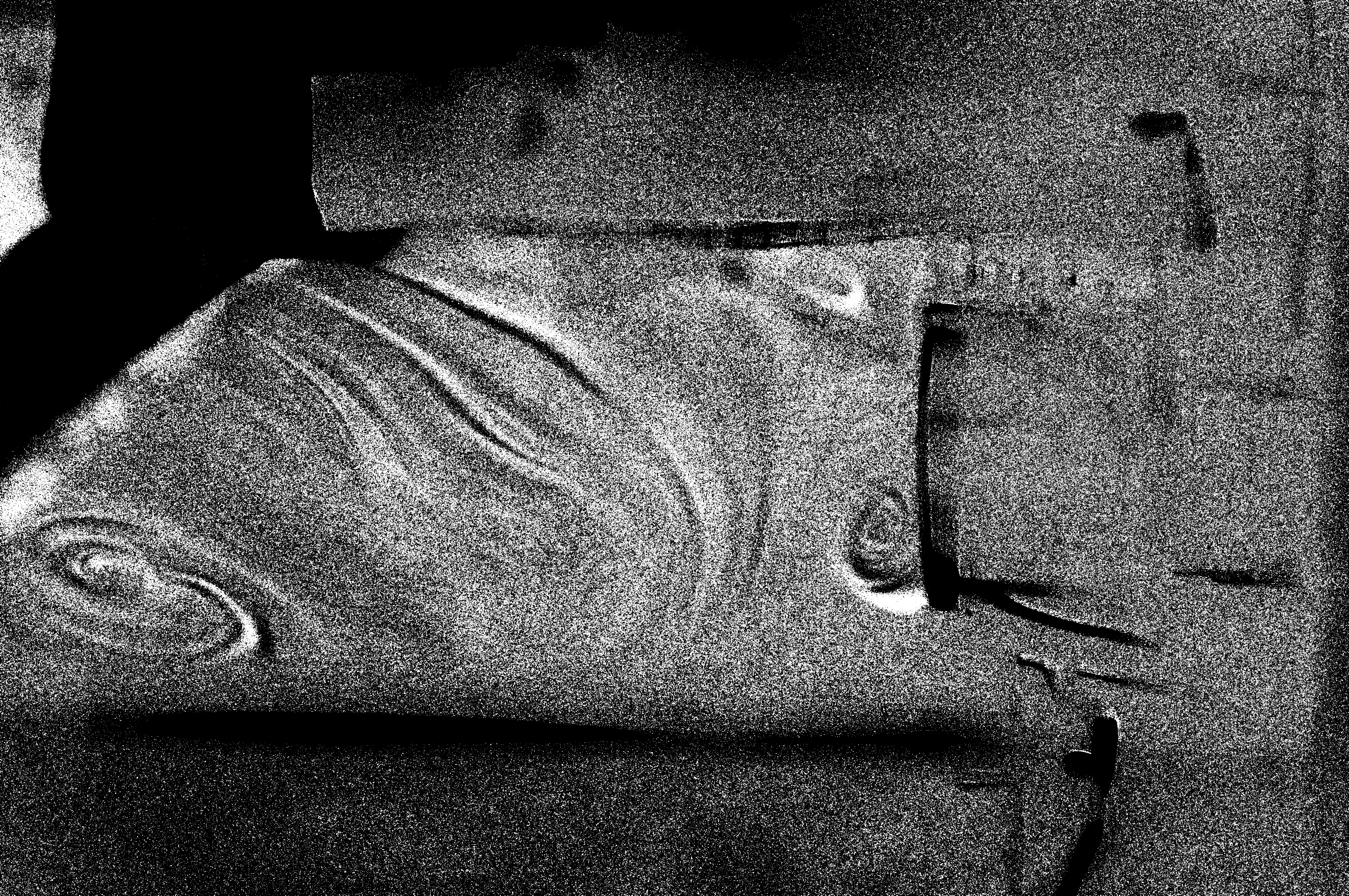
I was recently challenged to try to photograph sound. Here’s the result:

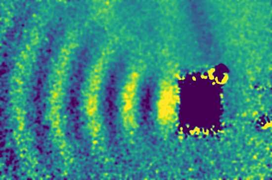
Looks pretty soundy! In this post I’ll try to explain what’s going on in that picture, talk about some of the things that didn’t work, and list some ideas to improve on this.

Schlieren photography

When light travels between regions of air with different densities it bends slightly (or refracts) — think of how a straw looks bent when it’s placed in a glass of liquid, but less extreme. These density variations can be caused by variations in temperature or pressure, so if we can find a way to visualise this bending we can use it to see temperature or pressure variations in air. Of course sound is just a pressure wave, so this works for our purposes too.

Schlieren photography is a family of techniques used to visualise these density variations.

The most well known technique involves a beam of collimated light passing through the air of interest. This is focused through a point across a knife edge which blocks light which has been bent. There are variations on this which don’t use collimated light, or use a colour filter instead of a knife edge, but the same principle applies.

With high resolution photography or large distances it’s possible to get similar results without any unusual optics. In Background Oriented Schlieren (BOS) imaging, a background pattern is photographed through the air of interest. The resulting image is shifted very slightly where there are density variations compared to a reference image. These shifts may be very small (fractions of a pixel) but can be extracted using techniques like optical flow or phase correlation.

I decided to try using BOS because of the simpler requirements and higher neat-factor.

The Setup

The setup for capturing the above above image is shown below.

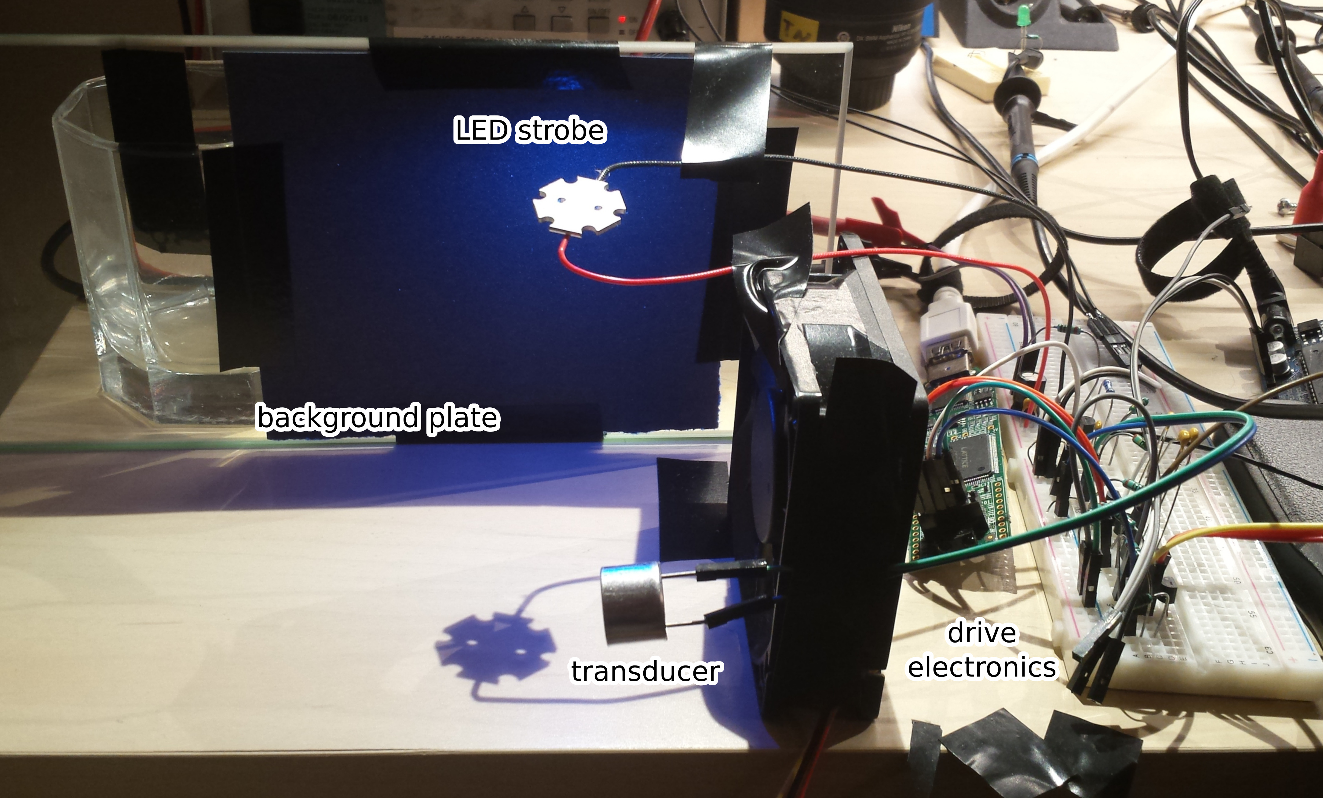
The ultrasonic transducer that is producing the sound is visible in the foreground. This is just a cheap thing from ebay, so I don’t have real specs. I decided to use ultrasound because it seemed like it would be easier to get to very high sound pressure levels (for example the muRata MA40B8S is rated at 120dB SPL at 10V) and would be less annoying in the process. It’s running at about 40kHz with a 25V square wave input.

The background plate is a piece of sandpaper, picked so that the grains are a few pixels across. This provides lots of edges across the entire frame.

The background plate is illuminated by an LED strobe light, with pulses synchronised to the sound from the transducer. Because the strobe and the sound are synchronised, when a photo is taken with a long exposure the pressure field seen by the camera is constant. The phase relationship between the sound and the strobe light can be varied to get images at varying phases.

Camera Setup

I used an 80mm lens on a DSLR with an APS-C sensor about 40cm away from the background plate, imaging a 12cm width. Normally large distances are used with BOS imaging so that both the background and foreground can be in focus, but this wasn’t possible because of the scale of the effect and the lenses that I had available.

Sequence and Processing

The above animation was derived from 8 acquisitions at with varying phases (pi/4 apart covering the whole circle), repeated 8 times for a total of 64 images.

Each frame in the animation is a comparison between the mean of the 8 images for one phase, and the mean of the 8 images that are pi out of phase. These two images contain exactly the opposite effects, so this is an easy way to get twice the signal compared to comparison with a single reference frame.

This averaging serves two purpose. It reduces noise in the image (and effectively gives higher brightness resolution), though this could be achieved with slower shutter speeds. More importantly it helps to average out small movements between frames caused by random vibrations, things settling, and vibrations from the camera shutter.

To find the displacements between two averaged images the Farneback optical flow algorithm [3] from opencv is used:

def get_shift(a, b):
    of = cv2.FarnebackOpticalFlow.create()
    of.setNumLevels(0)
    of.setWinSize(11)
    of.setPolyN(7)
    of.setPolySigma(0.9)
    of.setNumIters(15)
    of.setFlags(cv2.OPTFLOW_FARNEBACK_GAUSSIAN)
    return of.calc(a, b, None)[..., 0]

This is followed by a 51-pixel Gaussian blur, and normalisation by subtracting each images mean displacement.

These parameters were adjusted manually to get a result that looked nice. This is obviously not ideal, but it’s not that sensitive to the particular parameters used.

The most important parameter is to set the number of pyramid levels (NumLevels), which should be set depending on the expected amount of displacement — in this case we expect less than a pixel, so no pyramid is required. If this is set too high, then the algorithm can get confused at higher pyramid levels, where there is no longer enough structure to be able to accurately register the images.

The maximum displacement in the final image is 0.031 pixels, or about 1.6μm. The actual displacement is half of this because of the pi-out-of-phase comparison.

Misc. Details

Camera

Images were taken at f/8, ISO 100, 1/2s.

The aperture was chosen to minimise the blur of the foreground without introducing diffraction.

Most image sensors use a Bayer filter to produce a colour image. Because the strobe light is blue only a quarter of pixels receive any light, so the real resolution is halved compared to a regular full colour image. This means that the anti-aliasing filter is not as effective as for normal images, because it is likely designed to not cut off detail in the green channel (this seems to be true in practice too; that’s a post for another day).

To counter this the focus was set about 0.5mm in front of the background plate to reduce the contrast slightly. Using a green LED instead would have been a good idea.

Ultrasound

Ultrasonic transducers are usually designed to have a strong resonance around their frequency of operation. For example, see this image from the MA40B8S datasheet:

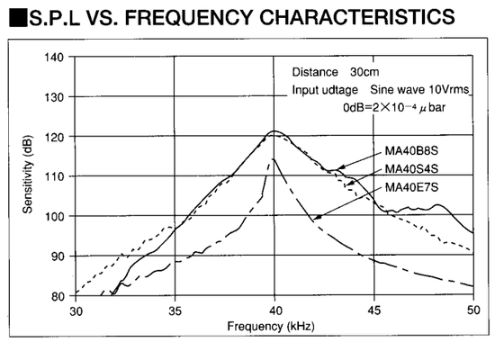
The frequency of that peak will vary depending on manufacturing tolerances, so the frequency was adjusted to get the highest SPL possible, as measured by another transducer.

Initially I was adjusting the frequency to maximise the input power, but this seemed to result in a lower frequency and more heating in the transducer, which was unexpected. More investigation required — perhaps this is caused by using a square wave input?

The specs for the transducers I’m using seemed to suggest that 10v would be the maximum input, but I was able to go to 25v without issue. Any higher and it looked like it was going into thermal runaway, but this might not have been a problem if I had been peaking the SPL rather than the input power.

When running about 400mW is used by the transducer and drive electronics, with minimal heating.

Strobe Light

At the very start of this project I tried to build a strobe light out of white LEDs, which did not work at all as the phosphor keeps glowing after the current is turned off.

Drive Electronics

The transducer and the strobe are both driven by an FPGA dev board (with a pile of interface electronics). This also has control of the camera shutter, allowing the whole thing to be sequenced by poking commands into the FPGA over a serial port from some python scripts.

Using an FPGA sounds a bit excessive, but it ended up being the easiest available option. Smaller microcontrollers tend to have a low clock speed and simplistic timer hardware, and while it probably would have been possible to implement on a teensy, the datasheet doesn’t exactly make it clear. Implementing a timer on an FPGA with all the features that I needed and serial control was pretty simple (using Migen, MiSoC and icestorm) and runs at 60MHz, giving plenty of resolution for adjustments.

For both the ultrasound and the strobe I initially had issues with BJT switching time: the strobe pulse wasn’t turning off quickly, and the halves of the half-bridge driving the transducer were overlapping, causing heating.

Both were solved by reducing the transistor base currents (by working resistor values out properly rather than guessing) and adding a speed-up capacitor. This stack exchange answer was very helpful, and contains a few other ideas that are worth knowing about.

Possible Improvements

Sound Source

It would be interesting to try other sources of sound and make some other neat images. For example:

regular loudspeakers or piezo elements
a phased array of ultrasonic transducers
reflections, or refractions
imaging of waves inside an ultrasonic delay line?

With some improvements there should be enough sensitivity to image sound (rather than ultrasound).

Image Capture

With more even illumination of the background plate the exposure could be increased, resulting in lower noise.

The sources of noise should be investigated in order to optimise the camera settings and capture sequence. The exposure time can be changed independently of all other settings by varying the strobe brightness — what would the ideal be? How many repeats of each phase are required? What is the best order to capture frames in?

Could the background plate be improved? If we’re only interested in horizontal displacements then vertical stripes might work better. The specular highlights from the sandpaper are not desirable, because they may cause aliasing or amplify/cancel the schlieren effect; a printed pattern may work better overall.

As above, using a green LED would have resulted in higher resolution images.

Image Processing

A more methodical approach should be taken to finding the best image processing algorithms. This would involve making an image sequence with known (or easily-knowable) offsets to evaluate different algorithms.

Other optical flow algorithms should be investigated. Ideally the optical flow algorithm should be aware of the particulars of this problem (very smooth flow, mostly horizontal displacements) so that it can better ignore noise. With the current background plate (which is quite peaky) ideally the optical flow algorithm should be able to ignore clipped pixels.

In theory phase correlation should work well on these kinds of images, as the displacements are very smooth, however I was not able to get any reasonable results — this should be investigated further.

Is it possible to integrate the averaging and optical flow steps? There will be slight shifts between the averaged images, which will cause blurring — if these images could be aligned before averaging then that could be reduced.

If a regular background plate is used then the technique shown in [0] may be appropriate.

Something Completely Different

I’d like to try building an optical schlieren imaging setup — mostly because it sounds fun, but it should be more sensitive. This really doesn’t need to be complicated; see for example [4], which is both simple and easy to understand.

What Didn’t Work

When I started this project I wanted to try to visualise the pressure field in air as directly as possible — without using schlieren imaging.

The plan was to have some smoke in a sound field be illuminated by a synchronised strobe light, then use image processing to amplify the change in brightness caused by the varying density of smoke.

This didn’t work. At all. I found that:

even if smoke looks uniformly dense and still, it probably isn’t
smoke tends to dissipate quite quickly; attempts to solve the first problem make this worse
when burned, different materials produce smoke that behaves quite differently

Essentially, I struggled to get a high enough signal-to-noise ratio.

Attempt 1

This was really quite silly. I used an ultrasonic humidifier that I had bought for another project to pass a stream of water droplets over an LED array. This was highly unsensible — even using 30s exposures and averaging over a few runs only resulted in noise.

Spraying water everywhere has self-evident soggy side-effects:

Thanks Alice. Thalice.

Attempt 2

The next approach was to enclose the whole thing in a jar to keep the smoke in. I tried both wood smoke and magic smoke from a resistor. Wood smoke tended to dissipate too quickly, and left condensation on the inside of the jar.

Magic smoke seemed to work better in both regards. This also made the set-up easier, since the whole thing can be assembled before the magic smoke is released from the resistor.

Even after it looks the smoke it has settled, there’s still quite a lot of swirling going on, which drowns out any signal in a cool-looking way:

Attempt 3

To try to smooth out the smoke I added a fan inside the jar. Initially I just ran this for 15s or so after making the smoke, which looked like it would be enough.

It wasn’t; this animation shows the smoke swirling, then fading to noise as the smoke dissipates:

Running the fan continuously during image capture solves the swirling problem, but causes the smoke to dissipate faster, and still didn’t reveal any sound.

For completeness, here’s a picture of the jar in all its glory:

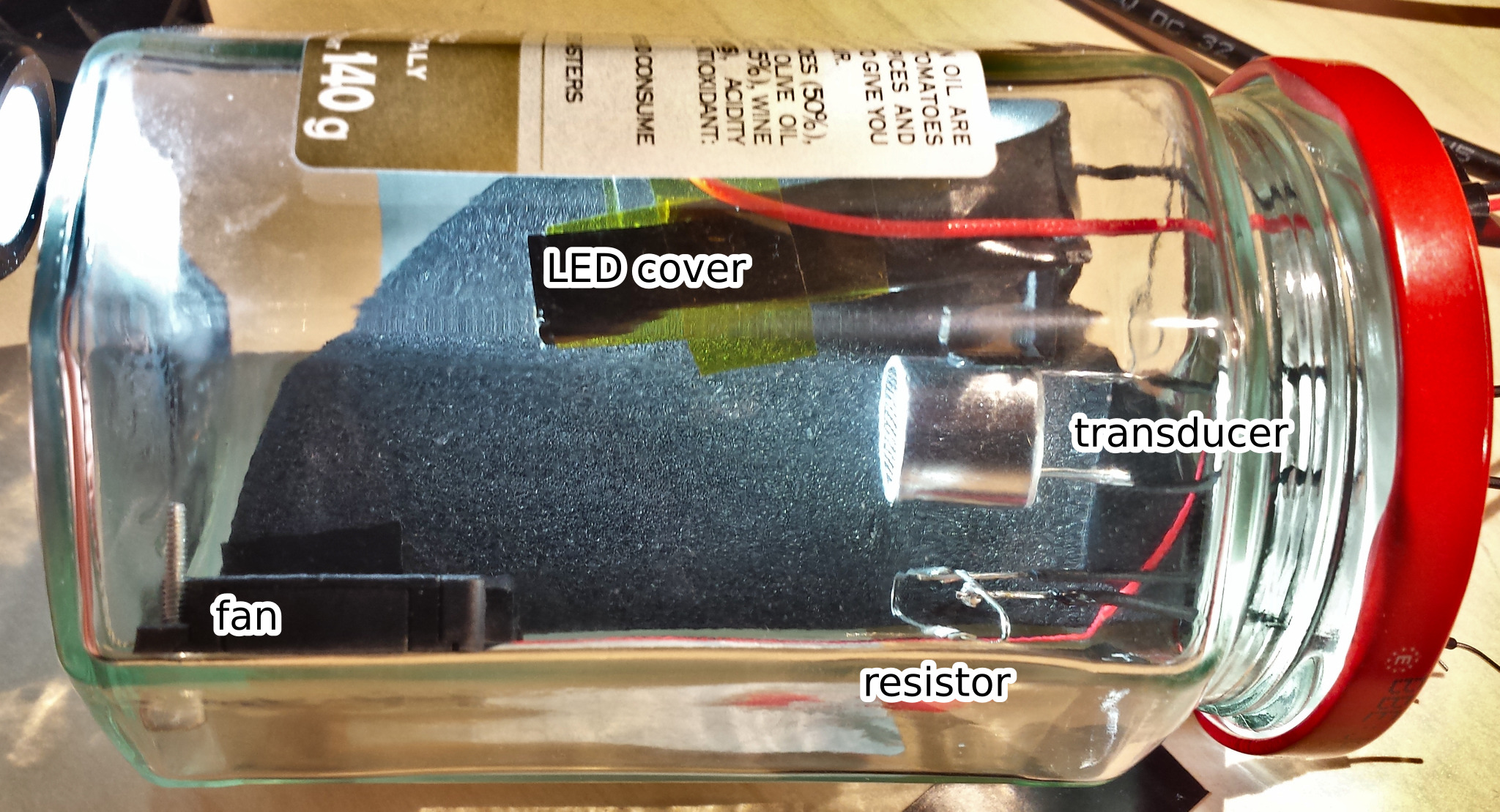
The LED is not visible as it’s covered in plastic which directs the light downwards in a thin sheet.

Conclusion

The smoke idea was fun to try, but ultimately a waste of time. Each attempt listed above is really many sub-attempts, tweaking variables to try to get something out of it — it took a long time and a lot of effort. It produced some cool looking images, but I don’t think I learned anything particularly useful from it.

Thankfully the electronics for the smoke and BOS setups are identical, so it only took an hour or so to get BOS working after playing with this for a month or so; I’m still surprised that this works as well as it does for such a simple setup.

Bibliography

[0]	(1, 2) Javh, J., Slavič, J. and Boltežar, M., 2017. The subpixel resolution of optical-flow-based modal analysis. PDF

[1]	Richard, H. and Raffel, M., 2001. Principle and applications of the background oriented schlieren (BOS) method. PDF

[2]	Yashiro, S., Takatsubo, J., Miyauchi, H. and Toyama, N., 2008. A novel technique for visualizing ultrasonic waves in general solid media by pulsed laser scan.

[3]	Farnebäck, G., 2003, June. Two-frame motion estimation based on polynomial expansion. PDF

[4]	Miller, V.A. and Loebner, K.T., 2016. Smartphone Schlieren. PDF